How to Estimate LLM API Cost Before Production
Monthly LLM API cost cannot be derived from a single prompt multiplied by a list price because production traffic involves variability in request volume, token distributions, model selection, caching, and retries. A practical estimation method converts workload assumptions into a cost range that accounts for these operational factors. This article provides a structured worksheet for building that range, anchored to measurable inputs rather than guesswork.
Why Single-Prompt Estimates Fail You in Production
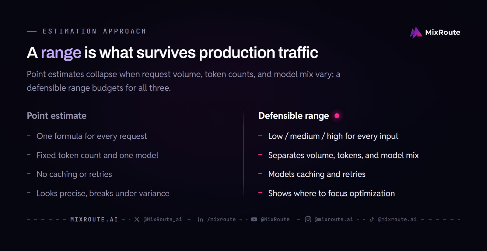
Multiplying one prompt by a list price ignores the variability in token usage, request volume, and operational factors like caching and retries. A point estimate looks precise but collapses the moment real traffic introduces variance. The goal of cost estimation is not a single number, it is a range you can defend to a finance team or a technical lead.
The problem with a single formula
A single formula assumes every request has the same token count, the same model, and the same failure rate. In production, prompt lengths vary by user, outputs vary by task, and the model mix changes as you add features. The formula also ignores caching, which can reduce cost by reusing prior responses, and retries, which multiply the number of calls.
What real workloads look like
A real workload has a distribution of token counts. Some requests are short, some are long, and the average rarely represents the median. The same applies to request volume, which fluctuates by hour, day, and feature release. A single prompt estimate cannot capture this distributional reality.
Why ranges beat point estimates
A range tells you the best case, the likely case, and the worst case. That boundary set is what you need for budgeting. It also lets you see which input has the largest impact on cost, so you know where to focus optimization effort.
Consider a scenario where your request volume spikes during peak hours. A point estimate that uses the average will understate the peak cost. A range that includes a high case for volume gives you the buffer needed for those spikes. Similarly, token counts can vary significantly. If you only use the average, you miss the tail that drives the bill. By building a low, medium, and high case for each input, you capture the full spectrum of possibilities. This is particularly important for budgeting because unexpected peaks can cause cost overruns. A range gives you a safety margin and helps you set aside contingency funds.
The Six Inputs That Drive Your LLM API Bill
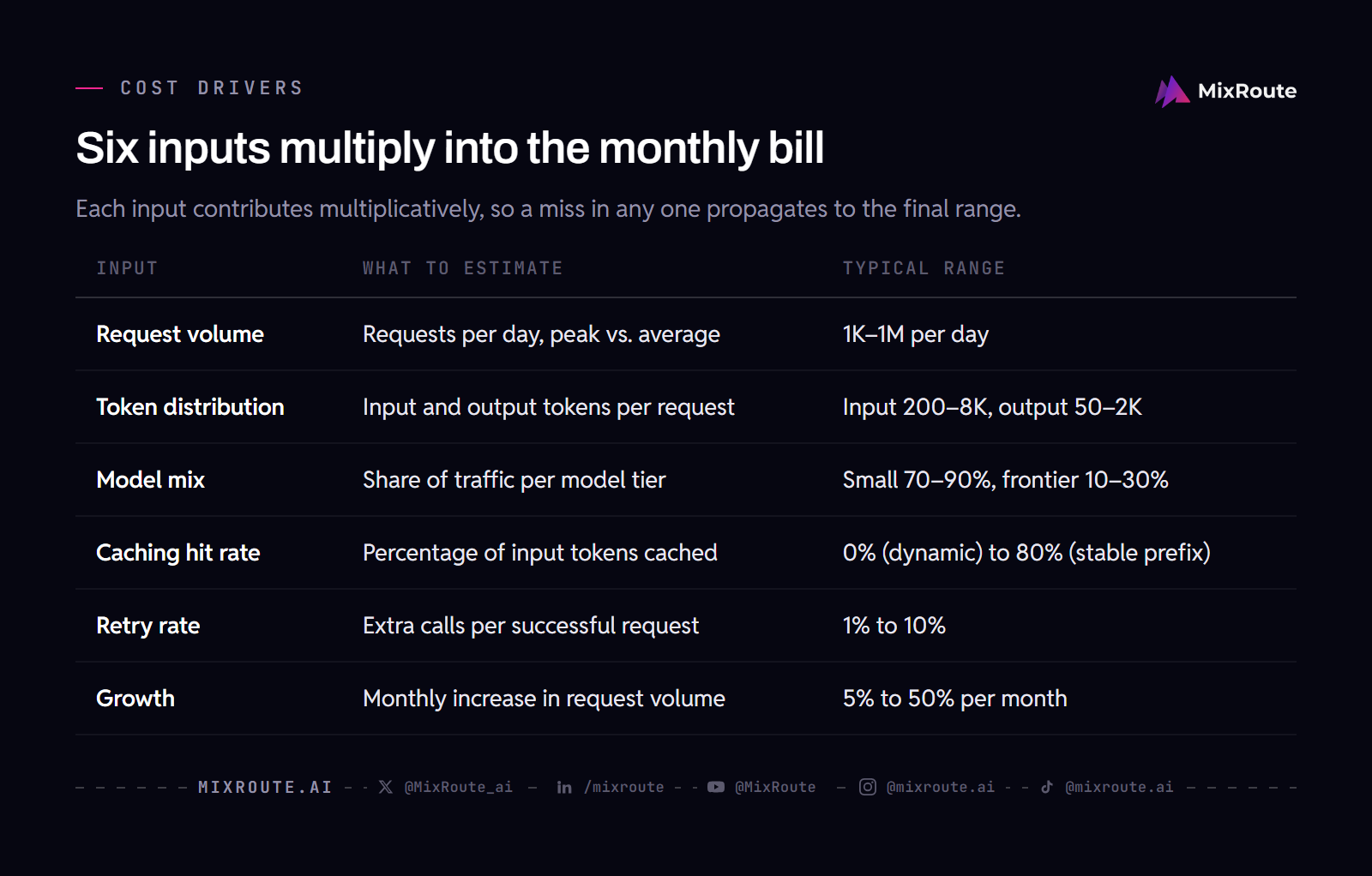
Request volume, token distributions per request, model mix, caching hit rate, retry rate, and growth rate over time are the six inputs that determine your monthly LLM API cost. Each one contributes multiplicatively, so an error in any input propagates to the final estimate. You need to estimate all of them, even if some start as rough assumptions.
Request volume: requests per day and peak
Estimate the average number of requests per day, then separately estimate the peak. Peak matters because it drives the need for rate limits or reserved capacity, and because some providers charge differently under sustained load.
Token distributions: input vs. output tokens
Providers charge different rates for input and output tokens, and output is typically more expensive. Separate these in your model. Estimate average input tokens per request and average output tokens per request, not total tokens, because the price ratio is rarely one to one.
Model mix: using multiple models
Most production systems route different tasks to different models. A simple classification may use a small model, while a complex reasoning task uses a frontier model. The mix matters because the price per token differs by an order of magnitude across models.
Caching: what it saves and when it helps
Prompt caching reuses the already-processed input prefix of a matching request and charges a reduced rate for those cached input tokens. It only helps for stable, repeated prompts. Conversational traffic with dynamic context caches poorly, while system prompts with fixed prefixes cache well.
Retries: extra calls due to failures
Retries add calls on top of your base request volume. A retry rate of 5 percent means 105 calls for every 100 successful requests. If the retry logic is aggressive, the rate can be much higher.
Growth: scaling from pilot to production
Growth changes request volume month over month. It also changes token distribution, because early adopters behave differently than a mass audience. Apply a monthly growth factor to the request volume, and re-examine the other inputs as the user base matures.
When setting your ranges, start with historical data if you have it. For a new feature, estimate the minimum and maximum plausible values for each input. For request volume, consider the number of active users and their usage patterns. For token distribution, think about the typical prompt and response lengths. For model mix, decide which tasks require a frontier model and which can use a smaller one. For caching, determine the proportion of requests that share a common prefix. For retries, set a range based on error rates observed in similar systems. The ranges you choose should be realistic, not overly optimistic or pessimistic. Also, consider the frequency of requests over time. Some features may have seasonal patterns. Include those in your volume estimate.
| Input | What to estimate | Typical range |
|---|---|---|
| Request volume | Requests per day, peak vs. average | 1K to 1M per day |
| Token distribution | Input and output tokens per request | Input: 200-8K, Output: 50-2K |
| Model mix | Share of traffic per model tier | Small 70-90%, Frontier 10-30% |
| Caching hit rate | Percentage of input tokens cached | 0% (dynamic) to 80% (stable prefix) |
| Retry rate | Extra calls per successful request | 1% to 10% |
| Growth | Monthly increase in request volume | 5% to 50% per month |
Ranges are illustrative estimates, not measured data.
How to Estimate Token Usage from Real Traffic
Use average tokens per request from logs, or estimate based on prompt length and expected outputs, and differentiate input and output tokens because pricing differs. The most reliable data source is your own traffic, but a new feature has no logs, so you build the estimate from first principles.
Measuring tokens from existing logs
If you already have a model in production, your logs contain token counts per request. Aggregate them into a distribution, not just a mean, and look at the percentiles. The p50 and p90 give you a range that is more honest than the average alone.
Estimating tokens for a new feature
For a new feature, estimate the typical user message length, the system prompt length, and the expected response length. Tokenization is not one character per token, so measure a few realistic examples using a tokenizer. You can also use the token documentation to convert characters to an approximate token count.
Handling variance with percentiles
Build a low, medium, and high case for token counts. The low case might be a short query with a brief answer, the high case a long document with a verbose response. This variance feeds directly into the final cost range.
To construct these cases, use percentiles: the low case at the 10th percentile, the medium at the 50th, and the high at the 90th. This gives a statistical view of token usage. The low case represents a minimal request, the high case a maximal one. The medium case should represent the typical request. Consider that some requests may be multi-turn, adding extra tokens per turn. Your cases should reflect the mix of request types and the variance in both input and output lengths. The percentiles should be based on your expected distribution, not on a uniform spread. If you have historical data, compute the actual percentiles.
The Effect of Caching and Retries on Cost
Caching reduces cost by charging a reduced rate for the already-processed input prefix when a new request matches it, but only if the prompt caches well, while retries multiply cost because each failed request may be retried, so factor in a retry rate. These two effects often cancel each other out, which is why you need to model both explicitly.
How prompt caching works
Prompt caching works by matching the input prefix of a new request against previously processed input. If the prefix matches, the provider charges a lower price for the cached portion. The cacheable portion is usually the system prompt and the static context, not the user turn.
Caching hit rate and cost impact
Hit rate is the percentage of input tokens that match a cached entry. A high hit rate on a long system prompt can cut the input cost substantially. A low hit rate, typical of highly dynamic conversations, saves almost nothing. Measure the hit rate from logs or estimate it based on how uniform your system prompt is.
Retry logic: how many extra calls to expect
Retry logic adds calls when a request fails due to rate limits, timeouts, or server errors. The retry rate is the number of extra calls divided by the number of successful calls. A rate limiting incident can push this rate up temporarily, so use a range rather than a fixed percentage.
Modeling retries in your estimate
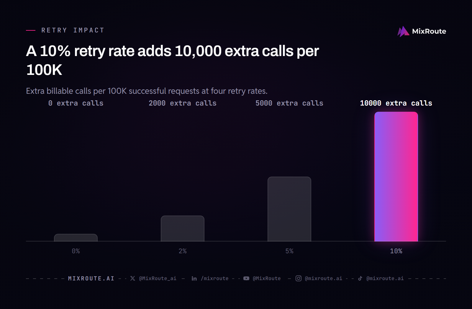
To model retries, multiply your base request count by the retry rate plus one. If you have 100,000 base requests and a 5 percent retry rate, you might pay for 105,000 requests. Add this multiplier before computing the final cost.
Retry logic also interacts with caching. A retried request may hit the cache if the same prompt is sent again, reducing the cost of the retry. Conversely, if the prompt changes between retries, the retry is a full-cost call. Moreover, a high retry rate can cause a feedback loop: more requests increase the chance of hitting rate limits, which then trigger more retries. To model this accurately, estimate the cache hit rate on retries. If your retries often use different prompts, the effective cache hit rate will be lower than for initial requests. You can model this by running separate calculations for the worst-case retry scenario and the best-case, then blending them.
| Retry rate | Effective call multiplier | Potential cost impact on 100K requests |
|---|---|---|
| 0% | 1.00x | 0 extra calls |
| 2% | 1.02x | 2,000 extra calls |
| 5% | 1.05x | 5,000 extra calls |
| 10% | 1.10x | 10,000 extra calls |
Projecting Cost Growth as You Scale
Multiply monthly request volume by a growth factor per month, and account for changes in token distribution and model mix as features evolve. Growth is not linear in practice, so your projection needs to separate the volume increase from the per-request cost change.
Linear vs. superlinear growth
Linear growth adds a constant number of requests each month. Superlinear growth, where each month adds more than the previous one, is common during a successful feature launch. Apply a compounding growth factor to the request volume, not an additive one.
Cost per request as a function of scale
Cost per request changes with scale in two ways. First, you may shift traffic to cheaper models as you learn which tasks need the expensive ones. Second, you may adopt caching or reserved capacity to lower the unit cost. The per-request cost is not fixed over time.
When to re-estimate
Re-estimate whenever you change the model mix, the prompt structure, or the retry logic. A monthly cadence is a good default. A major feature release or a provider price change is also a trigger for a fresh calculation.
When you re-estimate, do not just change the request volume. Each input has dependencies on the others. For example, moving to a larger model may increase the token count because responses are longer. Retry rates often rise after a feature release because of increased load. Caching effectiveness may improve as your system prompt stabilizes. Treat the estimate as a system of variables, not a list of independent numbers. Also, consider the time horizon. A longer projection requires different assumptions and wider ranges. Document the assumptions you used and the date, so you can track how accuracy improves over time.
Use a Cost Worksheet to Get a Range You Can Defend
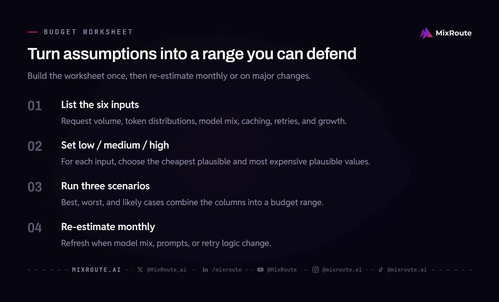
A structured worksheet that takes your assumptions and outputs a cost range, letting you compare scenarios and see the impact of each input, is the most effective way to build a defensible budget. The worksheet turns qualitative assumptions into a quantitative result, and it is reproducible.
Building the worksheet
Build the worksheet with rows for each of the six inputs: request volume, token distributions, model mix, caching hit rate, retry rate, and growth factor. For each input, create low, medium, and high columns. The low column represents the cheapest plausible outcome, the high column the most expensive.
Running scenarios
Run at least three scenarios. The best case combines low request volume, low tokens, a cheap model mix, high cache hit rate, and zero retries. The worst case combines the opposite. The likely case sits in between. The difference between the best and worst case is your budget buffer.
Connecting to the savings calculator
The worksheet is a manual process. If you want to see the range instantly, you can try the savings calculator and input the same assumptions. The calculator operationalizes the range so you can test scenarios without a spreadsheet.
Once you have the range, you can compare it against the pricing page to understand the fee structure. To reduce the cost, review the techniques in our guide to reduce LLM API costs. For a deeper look at the mechanism, read the prompt caching guide. Understanding the base unit is also important, which is explained in the token article. For a related scenario, see the analysis of AI agent costs.
FAQ
How can caching strategies impact monthly LLM API spend?
Caching reduces cost by charging a reduced rate for cached input tokens when a new request matches an already-processed prefix, but the impact depends on the hit rate and the cacheability of the prompt. A stable system prompt with an 80 percent hit rate cuts the input cost component significantly, while a dynamic conversation with a near-zero hit rate saves almost nothing. Model the hit rate explicitly because it directly scales the input token cost.
What adjustments should be made for retry logic in cost estimates?
Retries add extra calls, so apply a retry multiplier to your base request count. A 5 percent retry rate turns 100,000 requests into 105,000 potentially billable calls. The multiplier is calculated as one plus the retry rate, and it compounds with the token cost per request.
How to project cost growth based on scaling workload?
Apply a compounding monthly growth factor to the request volume, then adjust the token distribution and model mix as the feature evolves. The formula is new volume equals current volume multiplied by one plus the growth rate raised to the number of months. Cost then follows from the new volume and the revised per-request cost.
What is the difference between input and output token pricing?
Most providers charge more for output tokens, roughly 5x to 8x the input price on current flagship models, as checked on 2026-08-10 against the OpenAI, Anthropic and Google published API pricing pages. You must calculate the cost for each type separately because a single blended token price will bias the estimate. Multiply average input tokens by the input rate and average output tokens by the output rate, then sum the two.
How do model mix choices affect overall cost?
Using multiple models for different tasks balances cost and quality. Estimate the share of traffic for each model tier, then compute a weighted average cost per request. The weight is the percentage of requests that use that model, and the cost is that model’s price for the expected token count.
What fees does MixRoute charge on top of inference costs?
MixRoute charges a 0% top-up fee on all top-ups, and credits never expire. Smart Routing is optional and completely free, with no routing service fee. You only pay for actual usage of the selected model.
How accurate are cost estimates based on token counts alone?
Token counts are a starting point, but they are not the whole picture. Real costs vary with caching hit rates, retries, and the model mix. A range-based estimate that includes these factors is more realistic than a point estimate that assumes fixed tokens per request.